9.2 Parametric Assumptions

Once you have a likely statistical test in mind, the next question is whether the assumptions for that test are reasonable.

This is Step 2 in our 4-step hypothesis-testing process: check assumptions.

Checking assumptions can feel annoying at first. It can feel like an extra step between you and the analysis you actually want to run. But assumptions matter because they tell us whether the statistical test is likely to work the way it is supposed to work.

If assumptions are seriously violated, the p-value may be inaccurate, the effect size may be misleading, or the interpretation may not fit the data. That does not mean your study is ruined. It means you need to make a thoughtful decision.

Most of the inferential statistics we will use are , which means they rely on assumptions about the data. generally make fewer assumptions about the shape of the distribution, but they are not assumption-free.

Where assumption checks happen in jamovi

You may notice that jamovi gives you more than one way to check normality. You can check normality through Exploration → Descriptives, but you may also see normality checks built into specific inferential tests.

These are related, but they are not always testing the exact same thing. The Descriptives approach is checking the variable you selected. Some inferential tests check normality in a way that is more closely connected to the analysis you are running.

Most of the time, you will reach the same overall conclusion either way: normality looks reasonable, questionable, or clearly violated. But the exact values may differ slightly. That is okay.

For now, use Exploration → Descriptives to learn the basic idea of checking normality. Later, when you are running a specific inferential test, use the assumption checks built into that analysis when they are available.

This video recaps the main ideas in this section in another format.

Two Kinds of Assumptions

I find it helpful to separate assumptions into two broad types.

Design or data-structure assumptions are about whether the test matches the way the data were collected or measured. These include assumptions such as having a continuous dependent variable and independent observations. If these are wrong, you usually need a different test or a different analytic approach.

Distributional assumptions are about the shape or spread of the data. These include normality and homogeneity of variance. If these are violated, you may use a different version of the test, a non-parametric alternative, or another justified approach.

In this chapter, we will focus on four common assumptions:

The dependent variable is continuous.
Observations are independent when the test assumes independence.
The dependent variable is reasonably normally distributed.
Variances are reasonably similar across groups when the test assumes homogeneity of variance.

Assumption 1: Continuous Dependent Variable

Many parametric tests require a continuous dependent variable. This includes t-tests, ANOVA, correlation, and regression.

This means the dependent variable should represent a numerical amount where means and standard deviations are meaningful. Examples include exam scores, reaction time, depression scale scores, GPA, height, and time spent studying.

There is no formal statistical test for this assumption. Instead, you need to know:

what type of variable you are working with;
how the variable was measured;
whether a mean, standard deviation, and difference score would be meaningful.

This connects directly to Types of Variables and Levels of Measurement. A single Likert-type item is usually best understood as ordinal, but an average or total scale score created from several related items is often treated as continuous in practice.

If this assumption is violated

This is not really an assumption you “fix.” If the dependent variable is categorical, you probably chose the wrong test.

Return to Choosing the Correct Test and choose a test designed for a categorical dependent variable.

Assumption 2: Independence

The assumption of independence means that each observation is independent of the others. In plain language, one participant’s score should not determine, cause, or be linked to another participant’s score unless the statistical test is designed for related observations.

For example, if you randomly sample 100 students and measure each student’s test score once, those observations are probably independent.

However, observations may not be independent when:

the same participants are measured more than once;
participants are paired or matched;
students are nested within classrooms;
employees are nested within work teams;
multiple observations come from the same person.

This is why it matters whether you have a between-subjects or within-subjects design. If the same people are measured more than once, you should not use a test that assumes independent groups.

If this assumption is violated

Violating independence is usually a design issue, not a data-cleaning issue.

If the same participants are measured more than once, choose a within-subjects or repeated-measures test. If people are nested in classrooms, organizations, teams, or other groups, you may need more advanced methods such as multilevel modeling. We will not cover multilevel modeling in this course, but I want you to recognize why independence matters.

Assumption 3: Normality

The assumption of normality means that the dependent variable is reasonably normally distributed for the analysis you are conducting.

A is often called a bell-shaped curve. In a normal distribution, the data are symmetrically distributed around the mean, the mean and median are equal, skew and kurtosis are approximately 0, and we know the proportion of data that should fall within each standard deviation from the mean.

This is where students often ask, “How normal is normal enough?” Great question. Unfortunately, there is not one perfect answer.

Assumption checking is not a magic checklist where every method gives the same answer. It is a judgment process. You should use more than one piece of information and think about the severity of the violation, the sample size, and the test you plan to use.

Checking Normality

There are four main ways we will check normality in this course:

Visualize the distribution.
Test the skew and kurtosis.
Conduct a Shapiro-Wilk test.
Visualize the Q-Q plot.

You should use multiple methods when checking normality. These methods do not always agree perfectly. Personally, I tend to prioritize visual inspection and err on the side of caution. A statistical test can tell you whether a distribution differs from perfect normality, but real data are almost never perfectly normal.

A general way to check normality is through Exploration → Descriptives:

Move the dependent variable to the Variables box.
If you need to check normality within groups, move the grouping variable to Split by.
Under Statistics, select skewness and kurtosis if useful.
Under Plots, select histogram, density, box plot, and/or Q-Q plot.
Under Normality, select Shapiro-Wilk if available.

You learned how to describe continuous variables in Describing Continuous Variables and how to visualize continuous variables in Visualizing Continuous Variables. This is one reason those earlier chapters matter: descriptives and plots help you decide whether assumptions are reasonable.

Method 1: Visualize the Distribution

The first method is to visualize the distribution. In jamovi, go to Exploration → Descriptives and select a histogram, density plot, box plot, violin plot, and/or data points.

We visually inspect whether the distribution resembles a bell-shaped curve. We are not looking for perfection. We are looking for whether the shape seems reasonable enough for the test we plan to use.

In the following example, height appears approximately normally distributed.

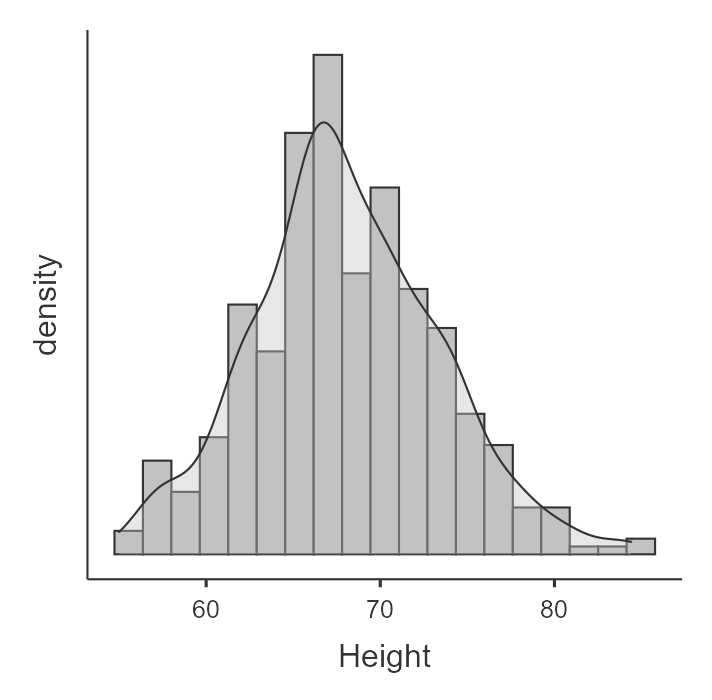
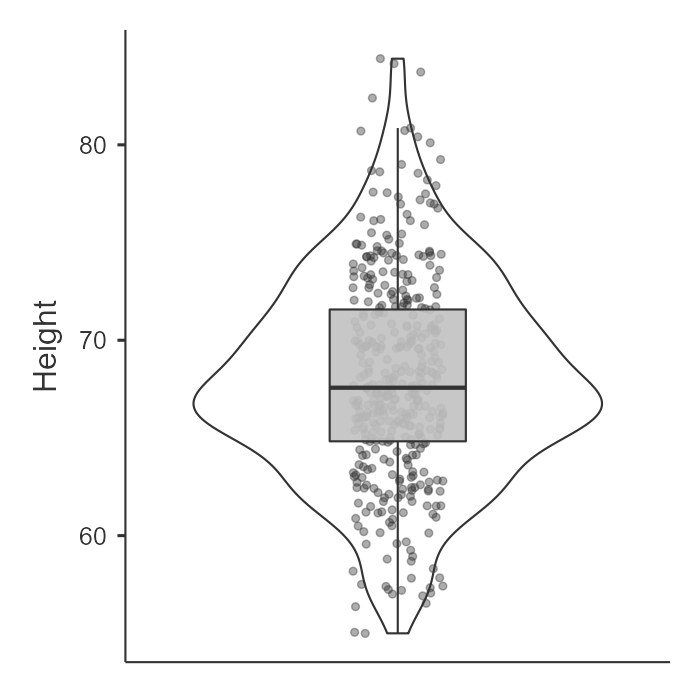
Histograms and density plots help us see the overall shape of the distribution. Box plots, violin plots, and data points can also help us notice skew, spread, and possible outliers.

Method 2: Test the Skew and Kurtosis

The second method is to examine skew and kurtosis.

In jamovi:

Go to Exploration → Descriptives.
Move your dependent variable into the Variables box.
Under Statistics, select skewness and kurtosis.

For our example of height, here are the skew and kurtosis values:

Descriptives	Height
Skewness	.230
Std. error skewness	.121
Kurtosis	.113
Std. error kurtosis	.241

To test skew and kurtosis, we calculate z-scores by dividing the value by its standard error:

Skew: .230 / .121 = 1.90
Kurtosis: .113 / .241 = .47

A common guideline is:

If |z| < 1.96, the skew or kurtosis value is not statistically significant at alpha = .05.
If |z| > 1.96, the skew or kurtosis value is statistically significant at alpha = .05.

Why 1.96?

The value 1.96 is the critical value of z when alpha is .05 and we have a two-tailed test. You do not need to memorize that for this course, but it explains why 1.96 often shows up when people are checking skew and kurtosis.

In this example, both values are less than 1.96 in absolute value, so skew and kurtosis do not suggest a serious violation of normality.

Method 3: Conduct a Shapiro-Wilk Test

The third method is to conduct a . This is a formal statistical test of normality.

In jamovi:

Go to Exploration → Descriptives.
Move your dependent variable into the Variables box.
Under Normality, select Shapiro-Wilk.

Interpretation:

If p > .05, the test does not provide evidence that the distribution differs from normality.
If p < .05, the test suggests the distribution differs from normality.

This can feel counterintuitive because we usually look for statistically significant results in inferential tests. For Shapiro-Wilk, we usually want a non-significant result because the null hypothesis is that the data are normally distributed.

Be careful, though. With very small samples, Shapiro-Wilk may miss meaningful non-normality. With very large samples, it may flag tiny deviations that do not matter much in practice. This is why you should not rely on Shapiro-Wilk alone.

Method 4: Visualize the Q-Q Plot

The fourth method is to visualize the Q-Q plot.

In jamovi:

Go to Exploration → Descriptives.
Move your dependent variable into the Variables box.
Under Plots, select Q-Q plot.

A compares the observed data to what we would expect if the data were normally distributed. We look for the points to fall reasonably close to the diagonal line.

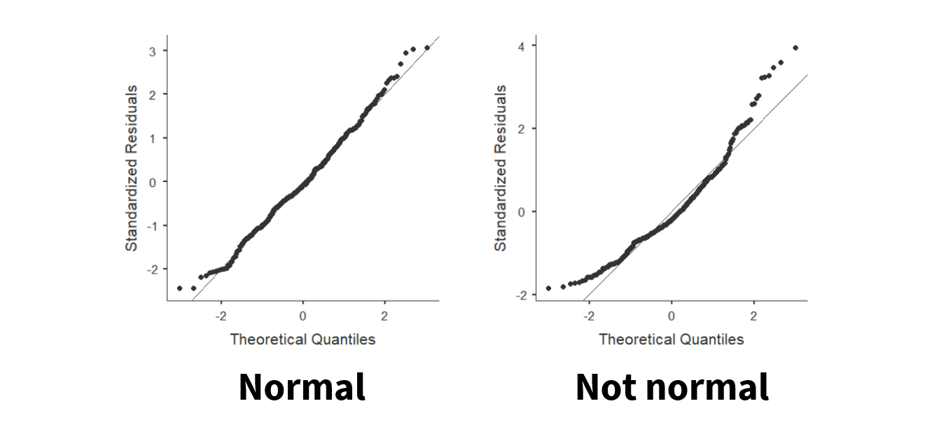
Focus primarily on the center of the distribution. Small deviations at the tails are common. Large, systematic deviations from the line suggest the data may not be normally distributed.

Here is a video by Alexander Swan on interpreting a Q-Q plot in jamovi:

If Normality Is Violated

First, check whether the violation is caused by data-entry errors, missing-value codes, or extreme outliers. If so, return to Cleaning and Preparing Data in jamovi.

If the data are genuinely non-normal, you may need to:

interpret the parametric test cautiously;
use a non-parametric alternative;
use a robust version of the test if available;
consider a transformation in more advanced work.

In this course, the most common move will be choosing the appropriate parametric or non-parametric test and explaining your decision. We will return to this in Violated Assumptions.

Assumption 4: Homogeneity of Variance

means the dependent variable has similar variability across groups of the independent variable.

This assumption applies when you are comparing groups on a continuous dependent variable, such as with an independent t-test or one-way ANOVA.

It might help to remember that homo means same and hetero means different. When variances are similar across groups, we have homogeneity of variance. When variances are very different across groups, we have heterogeneity of variance.

Normality vs. Homogeneity of Variance

Normality is about the shape of the dependent variable’s distribution.

Homogeneity of variance is about whether the spread of the dependent variable is similar across groups of the independent variable.

Checking Homogeneity of Variance

There are three main ways we will check homogeneity of variance in this course:

Visualize the distribution of the dependent variable across the groups of the independent variable.
Examine the variance values.
Conduct Levene’s test.

As with normality, these methods should be interpreted together. A graph may show that the group spreads look meaningfully different even before you look at a statistical test. Levene’s test may also be statistically significant in larger samples when the practical difference in spread is not very concerning. Use your judgment and be transparent about what you checked.

Method 1: Visualize the Distribution Across Groups

The first method is to visualize the distribution of the dependent variable across the groups of the independent variable.

In jamovi:

Go to Exploration → Descriptives.
Move the continuous dependent variable to the Variables box.
Move the categorical independent variable to the Split by box.
Select box plot, violin plot, and/or data points.

Large differences in spread across groups may suggest a violation.

You practiced this kind of graph in Visualizing Continuous Variables Across Groups.

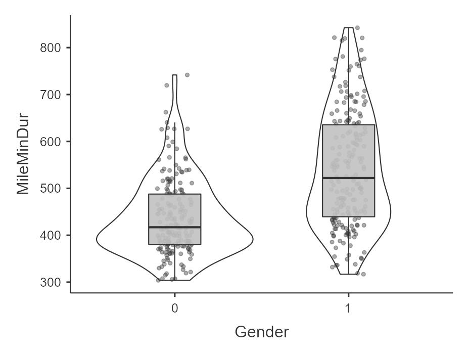
For example, here is an example of data that violates the assumption of homogeneity of variance. The dependent variable is mile duration in minutes, split by gender. The spread of scores for females, coded as 1, is much wider than the spread of scores for males, coded as 0. I am looking at the data points and violin plot to see the spread; the 1 looks wider whereas the 0 looks skinnier.

Method 2: Examine the Variance Values

The second method is to compare the variance values across groups.

In jamovi:

Go to Exploration → Descriptives.
Move the dependent variable to the Variables box.
Move the grouping variable to the Split by box.
Under Statistics, select variance.

Large differences in variance values suggest a possible violation of the assumption of homogeneity of variance.

Example:

Male variance in mile duration in minutes: 6796.20
Female variance in mile duration in minutes: 15401.55

Females have 2.26 times greater variance compared to males. Clearly, there is much greater variability for females than males for time it takes to run the mile.

Method 3: Conduct Levene’s Test

The third method is to conduct . Levene’s test is a formal statistical test of homogeneity of variance.

You will often find Levene’s test inside the inferential test menu. For example, for a one-way ANOVA, you can select the homogeneity test option.

In jamovi:

Go to ANOVA → One-way ANOVA.
Move your continuous dependent variable to the Dependent Variables box.
Move your categorical independent variable to the Grouping Variable box.
Check Homogeneity test.
Only look at Levene’s test for now; ignore the ANOVA results at this moment.

Interpretation:

If p > .05, the assumption is generally treated as met.
If p < .05, the assumption may be violated.

Here is the result of Levene’s test for the effect of gender on mile duration:

Levene’s	F	df1	df2	p
MileMinDur	41.33	1	381	< .001

Because the p-value is less than .05, this suggests that we violated the assumption of homogeneity of variance.

Why do we want Levene’s test to be non-significant?

Again, we usually want non-significant results here because the null hypothesis is that the variances are equal across groups.

If Homogeneity of Variance Is Violated

If homogeneity of variance is violated, the solution depends on the test.

For an independent t-test, you may use Welch’s t-test. For a one-way ANOVA, you may use Welch’s ANOVA. These versions adjust for unequal variances.

For repeated-measures designs, the assumption issues are different. For example, repeated-measures ANOVA has an assumption called sphericity. We will discuss that later when we get to ANOVA.

We will return to broader decision-making about violations in Violated Assumptions.

Regression Assumptions

Regression has additional assumptions, including linearity, homoscedasticity, independent errors, and normally distributed residuals. I am not going to teach those in depth here because they will make more sense when you learn regression.

For now, just know that regression is not assumption-free. We will return to regression-specific assumptions in Correlation and Regression.

Assumption Checking and Reporting

Assumption checking is not only about choosing the correct test. It also affects what you report.

If assumptions are met, you may simply report the planned test. If an assumption is violated and you use a different test, correction, or non-parametric alternative, readers need to know what you checked and what decision you made.

We will focus more on writing results clearly in Chapter 10.

Recapping Parametric Assumptions

Let’s summarize the four assumptions and generally how to test for them:

Continuous dependent variable
- Know your levels of measurement and make sure the dependent variable is continuous.
Independent scores on the dependent variable
- Know your research design and how the data were collected. Make sure that one participant’s data is not thought to affect another participant’s data.
Normal distribution of the dependent variable
- Visualize the distribution with a histogram and/or density plot of the dependent variable.
- Test the skew and kurtosis by calculating the z-scores.
- Test using the Shapiro-Wilk test.
- Examine the Q-Q plot for deviations from the diagonal line.
Homogeneity of variance
- Visualize the distribution with a box plot, violin plot, and/or data points, with the dependent variable split by the independent variable.
- Examine the variances of the dependent variable split by the independent variable.
- Test using Levene’s test.

Check Your Understanding

Which assumptions are determined conceptually rather than tested statistically?
What are the four ways we check normality in this course?
For normality, do we usually want statistically significant or non-significant Shapiro-Wilk results? Why?
What are the three ways we check homogeneity of variance in this course?
What does Levene’s test evaluate?